Understanding Self-Distillation and Privileged Information Distillation

Overview

This post covers recent works on self-distillation and privileged information distillation, including Shenfeld et al. (2026), Zhao et al. (2026), Hübotter et al. (2026), Ye et al. (2026), and Penaloza et al. (2026). The core idea behind these works is how to fix situations where the model cannot sample successful outcomes, assuming one does not have full access to a larger model but does have access to additional privileged information that can be added in context. We do not discuss in-depth results or how to mine or obtain privileged information, but note that common sources of privileged information are successful agentic trajectories (Penaloza et al., 2026), ground truth answers (Zhao et al., 2026), or self-reflection (Hübotter et al., 2026). Rather, we aim to build intuition for how these algorithms work, where they come from, and when their assumptions hold. Throughout, we favour gaining intuition over providing a complete nuanced view, using simplified 2D/3D visualizations of these algorithms to describe the core ideas.

We hope this blog is approachable to a broad audience assuming only a small background in reinforcement learning and its application to LMs. Regardless, we provide some supplemental reading for those interested.

@misc{penaloza2026privilegedinformationdistillationlanguage,
      title={Privileged Information Distillation for Language Models},
      author={Emiliano Penaloza and Dheeraj Vattikonda and Nicolas Gontier and Alexandre Lacoste and Laurent Charlin and Massimo Caccia},
      year={2026},
      eprint={2602.04942},
      archivePrefix={arXiv},
      primaryClass={cs.LG},
      url={https://arxiv.org/abs/2602.04942},
}

Reinforcement Learning as Variational Inference

The goal of RL is to maximize reward:

to obtain a target policy $\piStar$. Throughout this post we consider continuous rewards $R(y, x) \in \mathbb{R}$, where higher is always preferred.

A slightly different perspective treats RL as a variational inference problem where we define the target policy as a reward tilted distribution over outputs with prior $\pi_{\mathrm{ref}}$. In practice $\pi_{\mathrm{ref}}$ is typically the base model or an exponential moving average.

Since the partition function $Z$ makes direct inference intractable, we instead parameterize an approximate policy $\piSphi$ and minimize the reverse-KL divergence to $\piStar$. We use reverse-KL because we can only sample from $\piSphi$, not from $\piStar$

Minimizing this and dropping constants yields the standard KL-constrained RL objective

When $\beta = 0$ we recover the original reward-maximization objective. Otherwise, the KL term acts as a regularizer, encouraging the policy to stay close to the reference.

To illustrate this, consider the figure below where $\beta = 0$. The model quickly fits $\piStar$, but its entropy collapses onto a single high-reward mode.

When $\beta > 0$, the policy behaves similarly but drifts less from the reference policy $\pi_{\text{ref}}$ while preserving more entropy.

Both behaviors can be useful in different contexts. When entropy has collapsed, the model can reliably sample from a high-reward mode. When entropy is preserved, the model can potentially retain coverage over potentially higher-reward regions. Furthermore, preserving entropy can increase diversity, which can aid inference time scaling (Wang et al., 2023).

This tradeoff becomes more nuanced when distributions are multimodal (multiple peaks), which is the setting we consider for the remainder of this post.

Regardless, the choice of $\beta$ is largely task-specific and often decided via hyperparameter tuning (Shah et al., 2026).

Failures of Reinforcement Learning

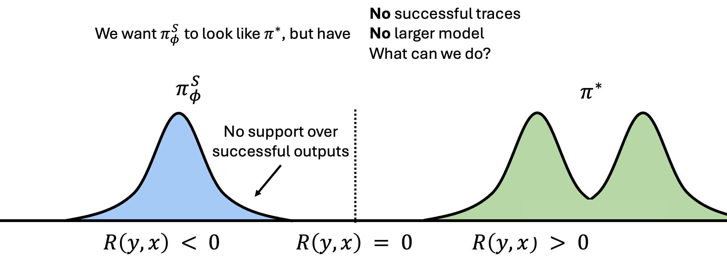
While RL has proven widely successful, specifically in LM reasoning, it relies on the policy $\piSphi$ being able to sample high-reward outputs. When the policy cannot produce any successful trajectories, there is no positive signal to reinforce.

For instance, consider the following setting:

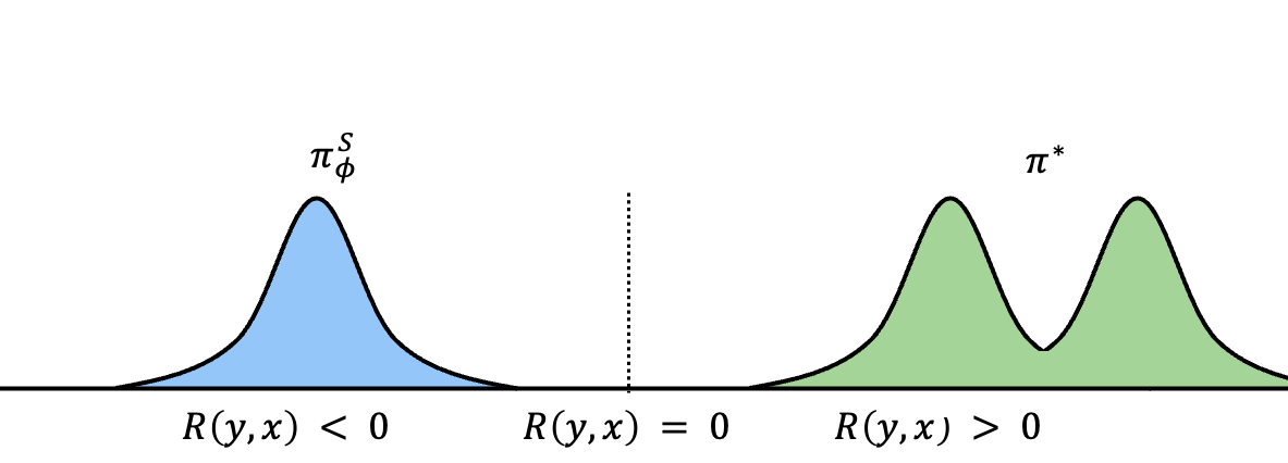
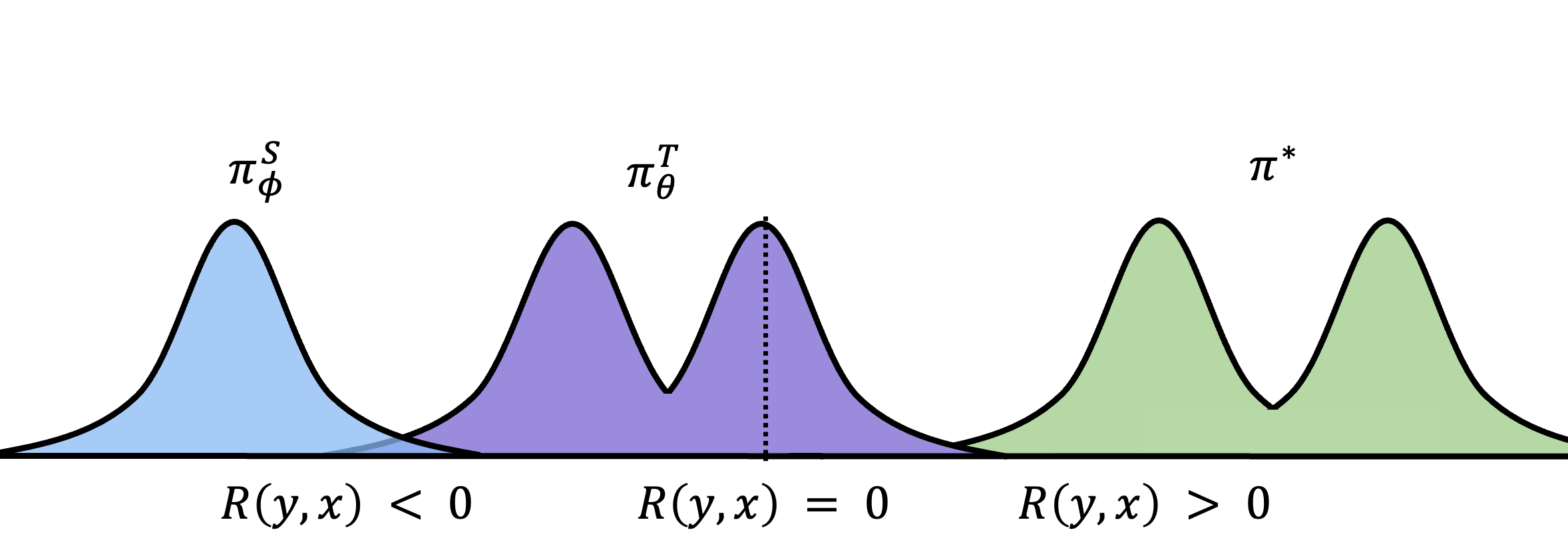
Notice that $\piSphi$ does not have support over correct trajectories, so applying RL in this setting would lead to the model only ever learning what not to do, never what to do. Without any high-reward samples to reinforce, it cannot bootstrap itself toward $\piStar$. While an LM technically has full support over the token space, making it theoretically possible to eventually sample a correct trajectory, this is practically infeasible.

These settings are common in practice. LMs often struggle to sample correct solutions to long-horizon agentic tasks and/or hard reasoning problems, so alleviating this could greatly improve performance.

Shaping a LM distribution by Conditioning

Although typical RL fails in these settings, LMs provide a useful property that can alleviate this problem. Unlike other ML systems, LMs can be freely conditioned on additional information. Notably, even a small amount of privileged information can enable models to succeed at tasks they previously could not. The figure below shows $\piTthetafull$, the same model now conditioned on privileged information $\mathbf{I}$, which we refer to as the teacher. Both start as the same model, but since training will change them differently, we use $\theta$ for the teacher and $\phi$ for the student.

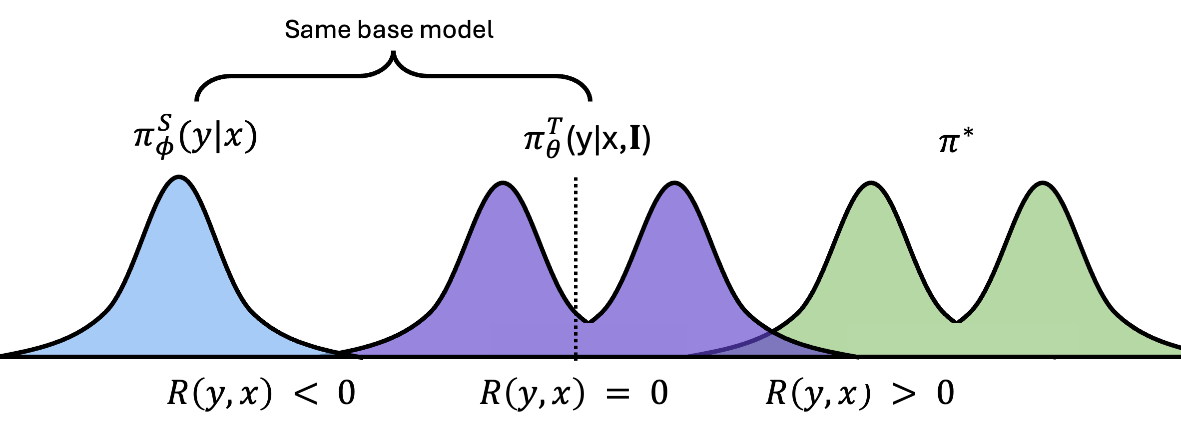
After contextualizing on $\mathbf{I}$, we see that the model can now sample successful traces. The only problem now is that we won’t have access to $\mathbf{I}$ at test time, since it is typically task-specific. So we need to find a way to transfer the information embedded within it to $\piSphi$, as this is the only deployable policy.

In the above example and for the remainder of the post, we assume that both $\piSphi$ and $\piTtheta$ share input prompts $x$ and outputs $y$ with the only difference between them being that $\piTtheta$ is additionally contextualized with $\mathbf{I}$. We further clarify that this is the case regardless of which policy is used for sampling. Allowing for this to happen in practice is fairly straight-forward, with the below diagram visualizing the how this is done:

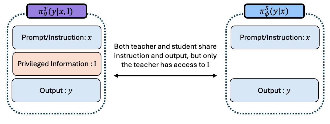
The remainder of this post explores different approaches to achieving this. Specifically, in settings where we assume $\piStheta$ and $\piTtheta$ are derived from the same base model.

1. SFT — supervised fine-tuning on teacher trajectories
2. Self-Distillation — matching the student to the teacher via reverse KL
3. Reward-Tilted Self-Distillation — reward tilted reverse KL
4. Fixing a Bad Teacher - Variational Expectation-Maximization — alternating between fitting the teacher and distilling to the student
5. $\pi$-Distill — joint teacher-student training with shared parameters

Supervised Fine-Tuning

By far the simplest and most popular way of transferring knowledge found in privileged information is through Supervised Fine-Tuning (SFT). This is equivalent to fitting forward-KL between the teacher policy $\piTtheta$ and the student $\piStheta$.

Since $\piTtheta$ is fixed, minimizing the forward-KL reduces to maximizing the expected log-likelihood under the student

Typically $\piTtheta$ is a larger model, but in our case it is the same model with added context $\mathbf{I}$.

While this approach is powerful, it is inherently limited by forward-KL being mode covering:

This can lead to the student outputting samples that are unlikely under the teacher, as forward-KL encourages $\piStheta$ to expand its support to cover all of $\piTtheta$ rather than accurately approximating it.

Self-Distillation via Reverse KL

A natural fix to the mode-covering behavior of forward-KL is to instead optimize reverse-KL, which is mode seeking. This idea comes from Agarwal et al. (2023), which shows that distilling on-policy can lead to significantly better performance and generalization on a variety of tasks when compared to SFT. When using $\piTthetafull$ as the teacher, this is referred to as self-distillation and optimizes the following objective

Optimizing this encourages the student to seek easy to fit modes of the teacher, which may not necessarily be optimal. This objective is the most widely used in recent works employed by Shenfeld et al. (2026), Hübotter et al. (2026) and Zhao et al. (2026), which has been shown to be a potent alternative to traditional SFT. We note that typically most works allow $\phi$ to equal $\theta$ as in Penaloza et al. (2026), be an exponential moving average as in Hübotter et al. (2026), Shenfeld et al. (2026), and Zhao et al. (2026), or simply be the base model.

Effectively, this objective acts similarly to the RL objective above:

Here we see that the student can appropriately fit the teacher’s mode, but this can lead to some suboptimal behavior where the policy fits a lower-reward mode of the teacher.

Reward-Tilted Self-Distillation

The main problem with pure self-distillation is its bias towards easier-to-fit modes, which may inherently be suboptimal. This comes from $\piTthetafull$ being the target distribution. A simple way to alleviate this is to define our target distribution $\piStar$ as a reward-tilted variant of $\piTthetafull$, which we use in Penaloza et al. (2026) and is partly used in Shenfeld et al. (2026):

Assuming $\theta$ is fixed with respect to $\piTtheta$, we can optimize the reverse-KL between the student and this tilted target. This yields the following objective

This objective explicitly rewards high-reward outputs while still matching the teacher’s structure.

Introducing this reward bias enables the student to fit higher-reward modes. Notice that this objective has the same form as the RL-as-inference objective, simply with the teacher as the prior instead of a fixed reference.

However, self-distillation in general assumes that the teacher is a fair approximation of $\piStar$, which can be unrealistic in many settings. For instance, in some cases $\piTtheta$ may not know how to properly leverage $\mathbf{I}$ to obtain the right answer.

Fixing a Bad Teacher - Variational Expectation-Maximization

One assumption that self-distillation relies on is that the teacher model $\piTtheta$ has support over high-reward regions, meaning $\piTtheta \approx \piStar$. While this is likely valid in many settings, it may not hold when even conditioning on $\mathbf{I}$ does not give the model sufficient coverage over high-reward regions.

For instance, see the figure below:

Here while $\piTtheta$ does have some coverage over successful outputs, most of its mass lies in the low-reward region. In this case, regardless of which algorithm we use, we are limited by the abilities of the teacher. To mitigate this, we can first train the teacher to approximate $\piStar$, putting us back in a setting where distillation is effective.

We can train the teacher via the same reward-tilted reverse-KL objective from before, but now defining the target as a reward-tilted variant of the student

Minimizing the reverse-KL between the teacher and $\piStar$ yields

Here $\text{sg}[\cdot]$ denotes stop-gradient, meaning the student is held fixed when updating the teacher. This objective encourages the teacher to maximize reward while not drifting too far from the student. Effectively, one part of the objective improves the teacher while the other prevents it from drifting too far from the student. Why does this matter? The student will eventually need to learn from the teacher’s samples. If those samples look nothing like what the student would generate on its own, the learning signal becomes noisy and hard to use. Keeping the teacher close ensures its samples stay on-policy for the student (Sutton & Barto, 2018) while also having higher reward. These properties encapsulate what makes up good training data, samples that the student can realistically learn from, but that are better than what it currently produces.

Using $J_{\text{Teacher}}$ we can make the teacher resemble $\piStar$, after which we can default back to distilling the knowledge via SFT (forward-KL).

Here KL-constrained RL first improves the teacher, allowing $\piTtheta$ to approximate $\piStar$ while collapsing onto a single mode since the KL constraint keeps it close to $\piSphi$. After improving $\piTtheta$ sufficiently, we can then use any distillation objective to fit $\piSphi$ onto $\piTtheta$. The fastest and most common is to use $J_{\text{SFT}}$ by drawing samples from the improved teacher $\piTtheta$ and using them to train $\piSphi$.

This approach can be viewed as variational expectation maximization, which is one of the most popular algorithms across machine learning and statistics (Dempster et al., 1977, Neal & Hinton, 1998, Bishop, 2006). Further, this algorithm is the one primarily used in Zhou et al. (2025). While it can improve over the base policy, in Penaloza et al. (2026) we show that it is inefficient and in many cases simply training the teacher suffices. Thus, one can greatly simplify the process by simultaneously training the teacher and student.

For interested readers, we provide a more formal framing of how the described procedure can be seen as variational EM:

$\pi$-Distill

While variational EM fits the teacher and student sequentially with different parameters for $\piStheta$ and $\piTtheta$, in Penaloza et al. (2026) we show this is inefficient and less effective. Rather, a simple solution is to allow $\piStheta$ and $\piTtheta$ to share parameters and jointly train the model, greatly simplifying the training process.

The teacher objective is the same as in Variational EM

Rather than training the student via naive SFT, we can use the same reward-maximizing objective as the teacher but via importance sampling. Since we want to distill the information from the teacher onto the student, which will not have access to $\mathbf{I}$ at deployment, we sample from the teacher and reweight:

We can then jointly optimize both objectives

A key component of $\pi$-Distill is its ability to modulate between the student and teacher objectives using $\alpha$. This allows for varying training configurations depending on the properties of the teacher.

• When $\alpha = 1$, optimization focuses entirely on the teacher, although the student may still improve through shared parameters.
• When $\alpha = 0$, training focuses on the student learning from the teacher’s current behavior. Interestingly, under certain conditions, parameter sharing can still lead to improvements in the teacher without explicit teacher updates.
• When $\alpha = 0.5$, both are optimized jointly. Shared parameters allow representations learned for using $\mathbf{I}$ to transfer to the student, while student updates keep those representations effective without $\mathbf{I}$.

To visualize $\pi$-Distill, we add an axis representing the KL between each policy and the base model $D_{\text{KL}}(\pi(\cdot) | \pi_{\text{base}}(\cdot \mid x))$. All three configurations can be used for learning, but each has different impacts on reward and divergence from the base model.

Teacher Training $\alpha = 1$

When $\alpha = 1$, only the teacher is being trained. This is similar to other work that explores conditional training with language models (Hatamizadeh et al., 2026, Shi et al., 2026).

Here we see the teacher improving and getting closer to $\piStar$. Training only the teacher incentivizes it to drift from the base model, with the KL term $D_{\text{kl}}\big(\piTthetafull \;|\; \text{sg}[\piSthetafull]\big)$ preventing it from straying too far from the student. We can also see that when $\piStheta$ and $\piTtheta$ share parameters $\theta$, training the teacher alone still helps the student improve.

In Section 7 of Penaloza et al. (2026), we show this generally works well, but one must be careful not to let the teacher collapse onto the student.

Student Training $\alpha = 0$

This is the opposite of the previous case. Here we only train the student via off-policy RL with traces from the teacher $\piTtheta$.

Training the student directly attracts it toward the teacher, and through shared parameters the teacher can also improve. Directly training on the teacher’s distribution is a significantly stronger attractor for the student compared to relying on implicit knowledge transfer from teacher-only training.

As shown in Section 7 of Penaloza et al. (2026), fitting teacher distributions can be difficult in higher-KL settings. This illustration depicts an ideal case.

Joint Training $ \alpha = 0.5$

Here the teacher is explicitly tasked with improving while the student is simultaneously tasked with approximating it. This creates a self-regularizing dynamic where the student actively tracks the teacher, preventing it from drifting too far.

Notice how the teacher can still drift but not as far as before. With explicit student training, we approximate the teacher directly, keeping both policies closer together than in teacher-only training.

In Section 7 of Penaloza et al. (2026), we show this configuration is the most stable, rarely performing the worst and being the most effective across settings.

Discussion

We hope this post serves as a useful starting point for building intuition about the different approaches to training with privileged information.

Many directions remain unexplored. For instance, $\pi$-Distill fits the student using off-policy traces from the teacher. In Penaloza et al. (2026) we show the success of this depends heavily on the properties of the privielged information, e.g., the utility or KL between student and teacher. Another approach is to do teacher training followed by self-distillation, which would be fully on-policy. This could lead to superior performance as reverse-KL is generally easier to fit, at the cost of a two-step procedure. Alternatively, one could jointly train them like in $\pi$-Distill, but this would require sampling from both the teacher and student simultaneously (since both are trained on-policy). Moreover other divergence metrics can be explored, Hübotter et al. (2026) is a good example, where they find Jensen Shannon Divergence can improve over naive reverse-KL optimization.

More effective types of privielged information mining are also a promising direction. Liao et al. (2026) is a good example of this, where conditioning on self-reflection allows agents to improve. Our work in Penaloza et al. (2026) suggests that for self-distillation, what matters most is the informativeness of the privielged information. If the teacher is too close to the student in terms of KL, they can collapse onto each other, making optimization harder. Mining helpful privielged information with sufficient but not excessive KL is a promising avenue.

Finally, recent work suggests that fitting policies to more off-policy data induces more forgetting. One can think of ways to slowly generate privielged information for questions that help the student improve without incentivizing the policy to substantially drift from itself. The work by Shenfeld et al. (2026) is a good example of this. Extending to different settings like harder agentic tasks where context can grow exponentially, or personalization, could yield interesting results.

References

[Zhou et al., 2025] Zhou, X., Liu, Z., Wang, H., Du, C., Lin, M., Li, C., Wang, L., & Pang, T. (2025). Variational Reasoning for Language Models. arXiv:2509.22637

[Shah et al., 2026] Shah, V., Obando-Ceron, J., Jain, V., Bartoldson, B., Kailkhura, B., Mittal, S., Berseth, G., Castro, P. S., Bengio, Y., Malkin, N., Jain, M., Venkatraman, S., & Courville, A. (2026). A Comedy of Estimators: On KL Regularization in RL Training of LLMs. arXiv:2512.21852

[Shenfeld et al., 2026] Shenfeld, I., Damani, M., Hübotter, J., & Agrawal, P. (2026). Self-Distillation Enables Continual Learning. arXiv:2601.19897

[Zhao et al., 2026] Zhao, S., Xie, Z., Liu, M., Huang, J., Pang, G., Chen, F., & Grover, A. (2026). Self-Distilled Reasoner: On-Policy Self-Distillation for Large Language Models. arXiv:2601.18734

[Hübotter et al., 2026] Hübotter, J., Lübeck, F., Behric, L., Baumann, A., Bagatella, M., Marta, D., Hakimi, I., Shenfeld, I., Kleine Buening, T., Guestrin, C., & Krause, A. (2026). Reinforcement Learning via Self-Distillation. arXiv:2601.20802

[Penaloza et al., 2026] Penaloza, E., Vattikonda, D., Gontier, N., Lacoste, A., Charlin, L., & Caccia, M. (2026). Privileged Information Distillation for Language Models. arXiv:2602.04942

[Agarwal et al., 2023] Agarwal, R., Vieillard, N., Stanczyk, P., Ramos, S., Geist, M., & Bachem, O. (2023). On-Policy Distillation of Language Models: Learning from Self-Generated Mistakes. arXiv:2306.13649

[Hinton et al., 2015] Hinton, G., Vinyals, O., & Dean, J. (2015). Distilling the Knowledge in a Neural Network. arXiv:1503.02531

[Vapnik & Vashist, 2009] Vapnik, V., & Vashist, A. (2009). A New Learning Paradigm: Learning Using Privileged Information. Neural Networks, 22(5-6), 544-557.

[Levine, 2018] Levine, S. (2018). Reinforcement Learning and Control as Probabilistic Inference: Tutorial and Review. arXiv:1805.00909

[Chen et al., 2026] Chen, J. C.-Y., Peng, B. X., Choubey, P. K., Huang, K.-H., Zhang, J., Bansal, M., & Wu, C.-S. (2026). Nudging the Boundaries of LLM Reasoning. arXiv:2509.25666

[Hatamizadeh et al., 2026] Hatamizadeh, A., Prabhumoye, S., Gitman, I., Lu, X., Han, S., Ping, W., Choi, Y., & Kautz, J. (2026). iGRPO: Self-Feedback-Driven LLM Reasoning. arXiv:2602.09000

[Liao et al., 2026] Liao, B., Dong, H., Xu, X., Monz, C., & Bian, J. (2026). Self-Hinting Language Models Enhance Reinforcement Learning. arXiv:2602.03143

[Sutton & Barto, 2018] Sutton, R. S., & Barto, A. G. (2018). Reinforcement Learning: An Introduction (2nd ed.). MIT Press. http://incompleteideas.net/book/the-book-2nd.html

[Wang et al., 2023] Wang, X., Wei, J., Schuurmans, D., Le, Q., Chi, E., Narang, S., Chowdhery, A., & Zhou, D. (2023). Self-Consistency Improves Chain of Thought Reasoning in Language Models. arXiv:2203.11171

[Dempster et al., 1977] Dempster, A. P., Laird, N. M., & Rubin, D. B. (1977). Maximum Likelihood from Incomplete Data via the EM Algorithm. Journal of the Royal Statistical Society: Series B, 39(1), 1-38.

[Neal & Hinton, 1998] Neal, R. M., & Hinton, G. E. (1998). A View of the EM Algorithm that Justifies Incremental, Sparse, and Other Variants. In Learning in Graphical Models (pp. 355-368). Springer.

[Bishop, 2006] Bishop, C. M. (2006). Pattern Recognition and Machine Learning. Springer.

[Shi et al., 2026] Shi, T., Chen, S., Jiang, B., Song, L., Yang, L., & Zhao, J. (2026). Experiential Reinforcement Learning. arXiv:2602.13949

[Hu et al., 2024] Hu, E. J., Jain, M., Elmoznino, E., Kaddar, Y., Lajoie, G., Bengio, Y., & Malkin, N. (2024). Amortizing Intractable Inference in Large Language Models. arXiv:2310.04363

[Ye et al., 2026] Ye, T., Dong, L., Wu, X., Huang, S., & Wei, F. (2026). On-Policy Context Distillation for Language Models. arXiv:2602.12275